Ice Dynamics, Part 3: Modeling Your Glacier

You are now in a position to model one of the glaciers you have been focusing on (choose a mountain glacier for the best results). We’ll start with the simplified model of a rectangular glacier flowing down a flat incline, but we’ll think about ways of expanding that model and then using OGGM’s built-in integration with the Rudolph Glacier Inventory (different from the World Glacier Monitoring Service database we’ve been using).

You can find and run the notebook from https://www.github.com/skachuck/clasp474_w2021.

# import oggm-edu helper package
import oggm_edu as edu

# import modules, constants and set plotting defaults
import matplotlib.pyplot as plt
plt.rcParams['figure.figsize'] = (9, 6)  # Default plot size

# Scientific packages
import numpy as np

# Constants
from oggm import cfg
cfg.initialize_minimal()

# OGGM models
from oggm.core.massbalance import LinearMassBalance
from oggm.core.flowline import FluxBasedModel, RectangularBedFlowline, TrapezoidalBedFlowline, ParabolicBedFlowline

# There are several numerical implementations in OGGM core. We use the "FluxBasedModel"
FlowlineModel = FluxBasedModel

2021-03-25 16:40:17: oggm.cfg: Reading default parameters from the OGGM `params.cfg` configuration file.
2021-03-25 16:40:17: oggm.cfg: Multiprocessing switched OFF according to the ENV variable OGGM_USE_MULTIPROCESSING
2021-03-25 16:40:17: oggm.cfg: Multiprocessing: using slurm allocated processors (N=1)

Basics

In order to set up the problem, you’ll need to consult the WGMS datasheets (sheet B) to find the highest and lowest elevation and the length. Make sure they’re all in meters! (Note, I’ve provided values appropriate for the Aletsch Glacier in the Swiss Alps so you can run through the whole notebook before performing data analysis of your own. Afterwards, and before answering the questions, enter the information for one of your glaciers.)

# Highest elevation (m)
HIEL = 3500
# Lowest elevation (m)
LOEL = 1510
# Glacier length (m)
LEN  = 24.7e3

We can use this information to get some approximate geometric parameters for the glacier, like the slope of the bed from the horizontal and the horizontal distance it covers.

print('Slope of bed: {} degrees'.format(np.rad2deg(np.arcsin((HIEL-LOEL)/LEN))))
BASE = np.sqrt(LEN**2 - (HIEL-LOEL)**2)
print('Distance of base: {} m'.format(BASE))

Slope of bed: 4.621146244185212 degrees
Distance of base: 24619.705522203145 m

Because we are going to want to experiment with what conditions change the glacier length, we want to extend the domain slightly, but we don’t want to change the slope of the bed, so we make sure that everything increases in proportion. If you get an error about the glacier exceeding the domain, change DOMSCALE to be bigger.

DOMSCALE = 2

top = HIEL
# Don't want the bottom to be below sea level, just yet
bottom = max(HIEL - DOMSCALE*(HIEL-LOEL), 0)
# get the actual scale 
actual_scale = (top-bottom)/(HIEL-LOEL)
print('Actual domain scale-up: {}'.format(actual_scale))

Actual domain scale-up: 1.7587939698492463

Glacier bed

# define horizontal resolution of the model:
# nx: number of grid points
# map_dx: grid point spacing in meters
map_dx = 100
nx = int(actual_scale*BASE/map_dx)
print('Number of 100 m grid points: {}'.format(nx))

Number of 100 m grid points: 433

# calculate the distance from the top to the bottom of the glacier in km
distance_along_glacier = edu.distance_along_glacier(nx, map_dx)
bed_h_slope, surface_h_slope = edu.define_linear_bed(top, bottom, nx)
initial_width = 300 #width in meters
# Now describe the widths in "grid points" for the model, based on grid point spacing map_dx
widths = np.zeros(nx) + initial_width/map_dx

The initial mass balance

Now extract the ELA for your glacier from sheet E and input it below

ELA = 2855 # equilibrium line altitude in meters above sea level

It’s a little harder to get the altitude gradient of the mass balance, but possible for some glaciers. Start out leaving this one alone, but come back to it to determine how sensitive the result is.

altgrad = 4 #altitude gradient in mm/m
mb_model_new = LinearMassBalance(ELA, grad=altgrad)

Running the Model

# Reinitialize the model
mb_flowline = RectangularBedFlowline(surface_h=bed_h_slope, bed_h=bed_h_slope, widths=widths, map_dx=map_dx)
model = FlowlineModel(mb_flowline, mb_model=mb_model_new, y0=0.)
# Year 0 to 1000 in 5 years step
yrs = np.arange(0, 1001, 5) 
# Array to fill with data
nsteps = len(yrs)
length_mb = np.zeros(nsteps)
vol_mb = np.zeros(nsteps)
# Loop
for i, yr in enumerate(yrs):
    model.run_until(yr)
    length_mb[i] = model.length_m
    vol_mb[i] = model.volume_km3
# I store the final results for later use
mb_glacier_h = model.fls[-1].surface_h

First, check the time evolution of the glacier.

f, (ax1, ax2) = plt.subplots(1, 2, figsize=(14, 5))
ax1.plot(yrs, length_mb, label='Mass Balance');
ax1.axhline(LEN, ls='--', c='k')
ax1.set_xlabel('Years')
ax1.set_ylabel('Length (m)');
ax1.legend()
ax2.plot(yrs, vol_mb);
ax2.set_xlabel('Years')
ax2.set_ylabel('Volume (km3)');

png

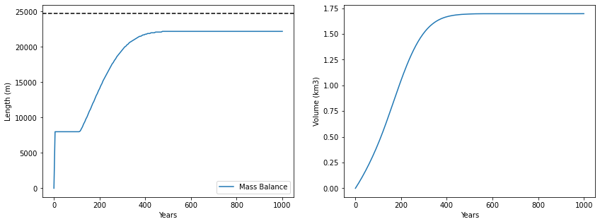
Q1 Has your modelled glacier come to equilibrium? How do you know? If not, run it for longer.

Now, we’re ready to compare with the data.

print('Modeled glacier length:  {} km'.format(length_mb[-1]/1000.))
print('Observe  glacier length: {} km'.format(LEN/1000.))

plt.axvline(LEN/1000., ls='--', c='k', label='Observed Length')
edu.glacier_plot(x=distance_along_glacier, bed=bed_h_slope, model=model, mb_model=mb_model_new, init_flowline=mb_flowline)

Modeled glacier length:  22.2 km
Observe  glacier length: 24.7 km

png

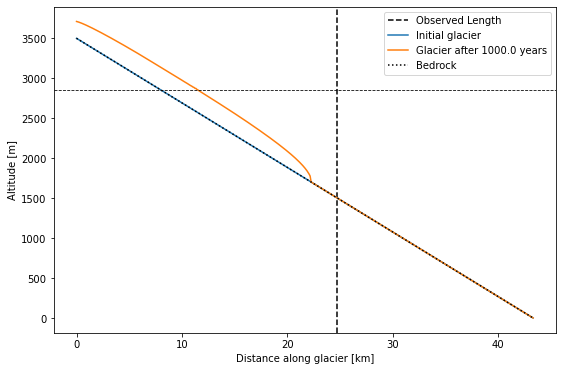
Q2 How does the modeled length of the glacier compare to the length you input at the very top (the dashed vertical line here)? What accounts for the difference?

Q3 Go back and evaluate the choices we made above: the bedrock top and bottom, the width, the mass balance altitude gradient. Change them a little and see how the modeled equilibrium length changes. First thing to do is to realize that the high altitude given is not for the bedrock, but for the ice surface. Try to decrease the high elevation HIEL so that the ice surface matches the observation. Now changes some other things. Remember that you can also change the temperature of the ice and the friction of the bed from the default OGGM values. Could getting those closer to the values experienced by the glacier decrease the distance between our modeled length and the observed length?

Alternatively, if you think your model and observation are a particularly good match, you could determine these parameters (temperature, friction, width, mass balance altitude gradient) by changing them until the model output matches the observation. This is called parameter fitting or model inversion and is a substantial branch of scientific methods.

Q3a (explorer) Perform a manual version of model fitting for the mass balance altitude gradient, especially if you can find some independent observations of it. Try to get as close to the observed length as you can by changing it. How close is your fitted parameter to the value you got from the observations?

Q4 Now consider the fundamental assumptions of our current model (particularly with how we’ve approximated the glacier). What are they and how might they affect our result?

Incorporating more information - The Randolph Glacier Inventory

OGGM is able to model glacier flowlines using geometries more closely resembling the ones we observe on the planet. The glacier outlines obtained from the Randolph Glacier Inventory are the reference dataset for global and regional applications in OGGM.

# this might take a couple of minutes!
from oggm import workflow, utils, graphics, tasks
from oggm.core import flowline

import pandas as pd
import geopandas as gpd

#utils.get_rgi_dir(version='62')  # path to the data after download
cfg.PATHS['working_dir'] = utils.gettempdir(dirname='OGGM-geometry', reset=True)

Select glaciers by their ID

Like the World Glacier Monitoring Service, each glacier in the RGI has a unique ID. Unfortunately, they are not the same. First, go through the notebook for the Altesch Glacier in the Swiss Alps to see how things work when they work. (For comparison with the flat incline model, you can use: HIEL = 3500; LOEL = 1510; LEN = 24.7e3 and run the flat incline model again.)

Then, before you answer the questions use the GLIMS viewer to search for your glacier and find its ID and enter it below. If things break, it’s possible the glacier you chose doesn’t have all the necessary data in the inventory. But never fear! When models break, it’s an opportunity to assess old assumptions, make new ones, and collect more observations!

# Enter the ID as a string (between ''). If you can't find an ID, 
# use RGI60-11.01450 for the Aletsch Glacier in the Swiss Alps
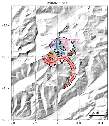
ID = 'RGI60-11.01450'

gdirs = workflow.init_glacier_directories([ID], from_prepro_level=3, prepro_border=80)
gdir = gdirs[0]

2021-03-25 16:40:28: oggm.workflow: init_glacier_directories from prepro level 3 on 1 glaciers.
2021-03-25 16:40:28: oggm.utils: Checking the download verification file checksum...
2021-03-25 16:40:29: oggm.workflow: Execute entity task gdir_from_prepro on 1 glaciers
2021-03-25 16:40:30: oggm.utils: /home/jovyan/.oggm_cache/download_cache/cluster.klima.uni-bremen.de/~oggm/gdirs/oggm_v1.4/L3-L5_files/CRU/centerlines/qc3/pcp2.5/no_match/RGI62/b_080/L3/RGI60-11/RGI60-11.01.tar verified successfully.

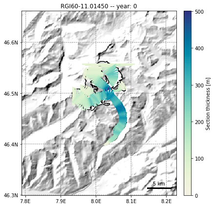
graphics.plot_domain(gdir, figsize=(8, 7))

png

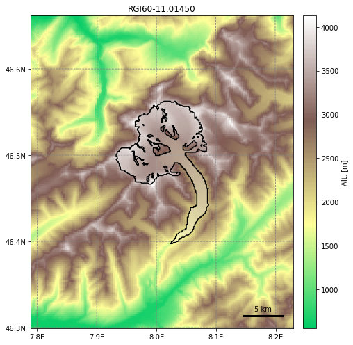
This is the geometry that the OGGM flowline model sees. The black line indicates the boundary of the glacier on the topography (downloaded from the Rudolph Glacier Inventory). These are considered fixed over time and do not evolve with the glacier, but thicknesses can evolve within this domain. OGGM will identify 6 flowlines from this particular example in the Swiss Alps, but we’ll only focus on the largest, which extends from the left lobe, down the trunk:

graphics.plot_centerlines(gdir, figsize=(8, 7), use_flowlines=True, add_downstream=True)

png

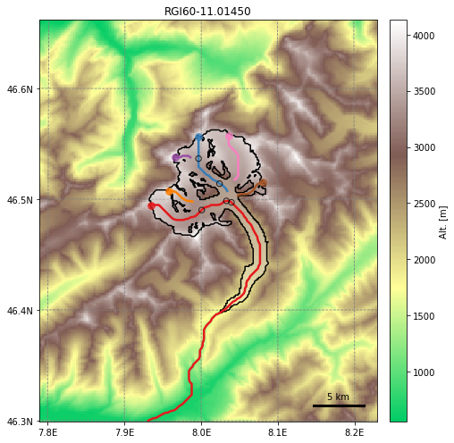
OGGM will then identify the width of every section of the flowline to generate a form factor for the ice dynamics and mass balance:

graphics.plot_catchment_width(gdir, corrected=True, figsize=(8, 7))

png

But before we can run the ice dynamics, we need to generate a mass balance model, which OGGM interpolates to this glacier from observations.

Temperature and Mass Balance Data

import xarray as xr
fpath = gdir.get_filepath('climate_historical')
ds = xr.open_dataset(fpath)
# Data is in hydrological years
# -> let's just ignore the first and last calendar years
ds.temp.resample(time='AS').mean()[1:-1].plot();

png

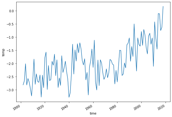
This climate data is called the “baseline climate” for this glacier. It will be used for the mass-balance model calibration, and at the end of this tutorial to generate preturbations to our model.

Now, let’s calibrate the mass-balance model for this glacier. The calibration procedure of OGGM is … original, but is also quite powerful. Read the doc page or the GMD paper for more details, and you can also follow the mass-balance calibration tutorial explaining some of the model internals.

The default calibration process is automated (see also local_t_star):

# Fetch the reference t* list and associated model parameters
params_url = 'https://cluster.klima.uni-bremen.de/~oggm/ref_mb_params/oggm_v1.4/RGIV62/CRU/centerlines/qc3/pcp2.5'
workflow.download_ref_tstars(base_url=params_url)

# Now calibrate
workflow.execute_entity_task(tasks.local_t_star, gdirs);
workflow.execute_entity_task(tasks.mu_star_calibration, gdirs);

2021-03-25 16:44:03: oggm.utils: /home/jovyan/.oggm_cache/download_cache/cluster.klima.uni-bremen.de/~oggm/ref_mb_params/oggm_v1.4/RGIV62/CRU/centerlines/qc3/pcp2.5/ref_tstars.csv verified successfully.
2021-03-25 16:44:03: oggm.utils: /home/jovyan/.oggm_cache/download_cache/cluster.klima.uni-bremen.de/~oggm/ref_mb_params/oggm_v1.4/RGIV62/CRU/centerlines/qc3/pcp2.5/ref_tstars_params.json verified successfully.
2021-03-25 16:44:03: oggm.workflow: Execute entity task local_t_star on 1 glaciers
2021-03-25 16:44:03: oggm.core.climate: (RGI60-11.01450) local_t_star
2021-03-25 16:44:03: oggm.core.climate: (RGI60-11.01450) local mu* computation for t*=1929
2021-03-25 16:44:03: oggm.workflow: Execute entity task mu_star_calibration on 1 glaciers
2021-03-25 16:44:03: oggm.core.climate: (RGI60-11.01450) mu_star_calibration

¡Important! The calibration of the mass-balance model is automated only for certain parameter combinations of the model - any change in the mass-balance model settings (e.g. the melt threshold, the precipitation correction factor, etc.) will require a re-calibration of the model (see the mass-balance calibration tutorial for an introduction to this topic).

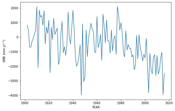
From there, OGGM can now compute the mass-balance for these glaciers. For example:

from oggm.core.massbalance import MultipleFlowlineMassBalance
mbmod = MultipleFlowlineMassBalance(gdir, use_inversion_flowlines=True)

import numpy as np
import matplotlib.pyplot as plt
years = np.arange(1902, 2017)
mb_ts = mbmod.get_specific_mb(year=years)
plt.plot(years, mb_ts); plt.ylabel('SMB (mm yr$^{-1}$)'); plt.xlabel('YEAR');

png

If your glacier has measured mass balance data, we can compare the computed mass-balance to the measured one:

mbdf = gdir.get_ref_mb_data()
mbdf['OGGM'] = mbmod.get_specific_mb(year=mbdf.index)
mbdf[['ANNUAL_BALANCE', 'OGGM']].plot(); plt.ylabel('SMB (mm yr$^{-1}$)');

png

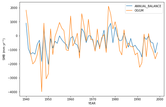
Q5 What do you think accounts for the difference between the observed and the modeled annual mass balance? Hint: it has to do with the fact that OGGM treats glacier outlines as fixed in time. But why does that matter?

Flowline geometry after a run with `FileModel`

Let’s do a run first. We set the initial time to 1975 because that’s the year of the datum I took from the World Glacier Monitoring Service and we run for 100 years.

TSTART = 1975 # Central year of the simulation
NYEARS = 100 # Number of years to run
years = range(0, NYEARS+1)

tasks.init_present_time_glacier(gdir)
tasks.run_constant_climate(gdir, nyears=NYEARS, y0=TSTART);

2021-03-25 16:44:05: oggm.core.flowline: (RGI60-11.01450) init_present_time_glacier
2021-03-25 16:44:05: oggm.core.flowline: (RGI60-11.01450) run_constant_climate
2021-03-25 16:44:05: oggm.core.flowline: (RGI60-11.01450) flowline_model_run

We use a FileModel to read the model output:

fmod = flowline.FileModel(gdir.get_filepath('model_run'))

A FileModel behaves like a OGGM’s FlowlineModel:

fmod.run_until(0)  # Point the file model to year 0 in the output
graphics.plot_modeloutput_map(gdir, model=fmod)  # plot it

png

fmod.run_until(NYEARS)  # Point the file model to year 100 in the output
graphics.plot_modeloutput_map(gdir, model=fmod)  # plot it

png

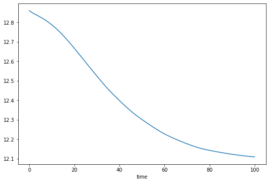
# Bonus - get back to e.g. the volume timeseries
fmod.volume_km3_ts().plot();

png

Because this glacier has a more complicated geometry, we use a differeny way of storing the data, that comes from the pandas package, which you can look into if you’re interested. We create a table of the main flowline’s grid points location and bed altitude (this does not change with time):

fl = fmod.fls[-1]  # Main flowline
i, j = fl.line.xy  # xy flowline on grid
lons, lats = gdir.grid.ij_to_crs(i, j, crs='EPSG:4326')  # to WGS84

df_coords = pd.DataFrame(index=fl.dis_on_line*gdir.grid.dx)
df_coords.index.name = 'Distance along flowline'
df_coords['lon'] = lons
df_coords['lat'] = lats
df_coords['bed_elevation'] = fl.bed_h

Now store a time varying array of ice thickness, surface elevation along this line:

df_thick = pd.DataFrame(index=df_coords.index)
df_surf_h = pd.DataFrame(index=df_coords.index)
df_bed_h = pd.DataFrame()
for year in years:
    fmod.run_until(year)
    fl = fmod.fls[-1]
    df_thick[year] = fl.thick
    df_surf_h[year] = fl.surface_h

f, ax = plt.subplots()
df_surf_h[[0, int(NYEARS/2), NYEARS]].plot(ax=ax);
df_coords['bed_elevation'].plot(ax=ax, color='k');
plt.title('Ice thickness at three points in time');

png

We can extract the glacier length over time just as we have in the past:

length_oggm = np.zeros_like(years)
for year in years:
    fmod.run_until(year)
    fl = fmod.fls[-1]
    length_oggm[year] = fl.length_m

plt.plot(years, length_oggm)
plt.xlabel('YEAR'); plt.ylabel('Length (m)');

png

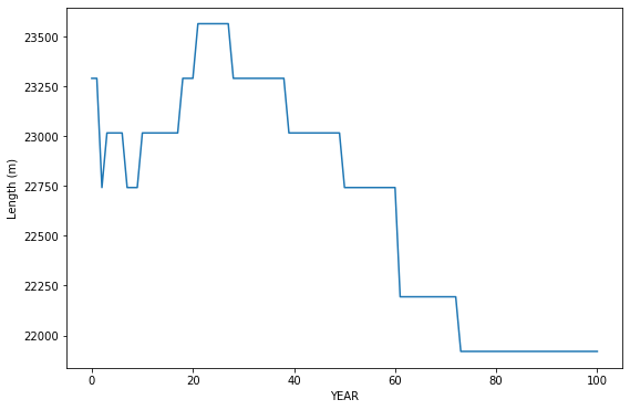
Q6 Is this glacier in equilibrium? We or why not?

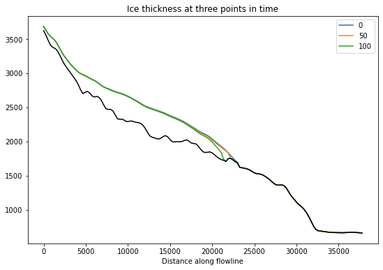
If you still have your flat bed run saved in memory, you can plot it on top of the mode complex model here:

f, ax = plt.subplots()
df_surf_h[[0, 50, 100]].plot(ax=ax);
df_coords['bed_elevation'].plot(ax=ax, color='k');
plt.title('Ice thickness at three points in time');

#print('Modeled glacier length: {} km'.format(length_mb[-1]/1000.))
ax.axvline(LEN, ls='--', c='k', label='Observed Length')

ax.plot(distance_along_glacier*1000, bed_h_slope, alpha=0.75)
ax.plot(distance_along_glacier*1000, model.fls[-1].surface_h, alpha=0.75)

Q7 Contrast the two models. How does the bed elevation differ between them? How do the thicknesses? The lengths?

Temperature Sensitivity

We can now run the same glacier flowline model, but biasing the temperature up and down by half a degree celsius (see temperature_bias in the function call).

workflow.execute_entity_task(tasks.run_constant_climate, gdirs, nyears=100,
                             temperature_bias=0.5,
                             y0=1975, output_filesuffix='_p05');
workflow.execute_entity_task(tasks.run_constant_climate, gdirs, nyears=100,
                             temperature_bias=-0.5,
                             y0=1975, output_filesuffix='_m05');

2021-03-25 16:46:00: oggm.workflow: Execute entity task run_constant_climate on 1 glaciers
2021-03-25 16:46:00: oggm.core.flowline: (RGI60-11.01450) run_constant_climate_p05
2021-03-25 16:46:01: oggm.core.flowline: (RGI60-11.01450) flowline_model_run_p05
2021-03-25 16:46:31: oggm.workflow: Execute entity task run_constant_climate on 1 glaciers
2021-03-25 16:46:31: oggm.core.flowline: (RGI60-11.01450) run_constant_climate_m05
2021-03-25 16:46:31: oggm.core.flowline: (RGI60-11.01450) flowline_model_run_m05

We’ll save things out in yet another way now. They all work, so pick and choose from the codes provided here.

dsp = utils.compile_run_output(gdirs, filesuffix='_p05')
fmodp = flowline.FileModel(gdir.get_filepath('model_run', filesuffix='_p05'))
dfp_coords = pd.DataFrame(index=fmodp.fls[-1].dis_on_line*gdir.grid.dx)
dfp_coords['bed_elevation'] = fmodp.fls[-1].bed_h
dfp_thick = pd.DataFrame(index=df_coords.index)
dfp_surf_h = pd.DataFrame(index=df_coords.index)
dfp_bed_h = pd.DataFrame()
for year in range(0, 101):
    fmodp.run_until(year)
    flp = fmodp.fls[-1]
    dfp_thick[year] = flp.thick
    dfp_surf_h[year] = flp.surface_h

dsm = utils.compile_run_output(gdirs, filesuffix='_m05')
fmodm = flowline.FileModel(gdir.get_filepath('model_run', filesuffix='_m05'))
dfm_coords = pd.DataFrame(index=fmodm.fls[-1].dis_on_line*gdir.grid.dx)
dfm_coords['bed_elevation'] = fmodm.fls[-1].bed_h
dfm_thick = pd.DataFrame(index=df_coords.index)
dfm_surf_h = pd.DataFrame(index=df_coords.index)
dfm_bed_h = pd.DataFrame()
for year in range(0, 101):
    fmodm.run_until(year)
    flm = fmodm.fls[-1]
    dfm_thick[year] = flm.thick
    dfm_surf_h[year] = flm.surface_h

2021-03-25 16:47:02: oggm.utils: Applying global task compile_run_output on 1 glaciers
2021-03-25 16:47:02: oggm.utils: Applying compile_run_output on 1 gdirs.
2021-03-25 16:47:03: oggm.utils: Applying global task compile_run_output on 1 glaciers
2021-03-25 16:47:03: oggm.utils: Applying compile_run_output on 1 gdirs.

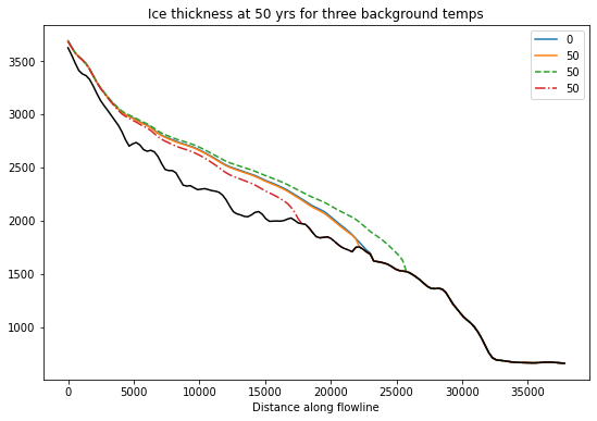
f, ax = plt.subplots()
df_surf_h[[0, 50]].plot(ax=ax);
dfm_surf_h[[50]].plot(ax=ax, ls='--');
dfp_surf_h[[50]].plot(ax=ax, ls='-.');
dfp_coords['bed_elevation'].plot(ax=ax, color='k');
plt.title('Ice thickness at 50 yrs for three background temps');

png

length_oggm_m = np.zeros_like(years)
for year in years:
    fmodm.run_until(year)
    fl = fmodm.fls[-1]
    length_oggm_m[year] = fl.length_m
    
length_oggm_p = np.zeros_like(years)
for year in years:
    fmodp.run_until(year)
    fl = fmodp.fls[-1]
    length_oggm_p[year] = fl.length_m

plt.plot(years, length_oggm, label='Control Run')
plt.plot(years, length_oggm_m, label='Colder')
plt.plot(years, length_oggm_p, label='Warmer')
plt.xlabel('YEAR'); plt.ylabel('Length (m)');
plt.legend();

png

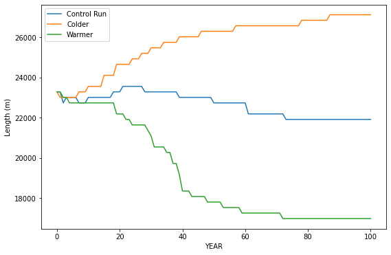
Q8 Compare these evolution of lengths to the timeseries of mass balance and length from the data you have from World Glacier Monitor Service. Do the trends in the data follow any of these modeled trends?